Effect size, Sample size, Significance and Power in Hypothesis Testing
When doing hypothesis testing, there are four related concepts one should keep in mind: effect size, sample size, significance threshold and power. Most people aware of hypothesis testing are likely aware of sample size and the significance threshold (typically denoted α), however all four are related and influence the cost and results of the test.
Definitions and relationships
Significance threshold: the threshold on the p-value of a test to reject the null hypothesis. The significance threshold is meant to control the type I error, the probability we reject a null hypothesis when we shouldn’t have. If we ran this experiment many times, the significance threshold is the probability (p(D|Null)) of seeing a result at least as extreme assuming the null hypothesis.
The scientific community has recently been pushing for a more nuisanced look at hypothesis testing in which thresholds of significance are not used. This post will indirectly shed some light on why this is important
Sample size: Number of samples taken in the experiment. Increasing samples allows for detecting increasingly small effect size. This may not be what is desired
Power: probability of rejecting a false null hypothesis. If the null hypothesis is actually false, will we reject it?
Effect size: How large an effect we observed. This value doesn’t increase with increasing sample size as the test statistic does. Larger effect size implies a more interesting or compelling result. If we are trying to detect if two samples share the same mean, it is the difference in the means divided by the standard deviation of the pooled samples. If we are trying to detect if a dice is fair, it is the chi squared statistic divided by n.
Visualizing the relationships
Using python and statsmodels, we can see exactly how these relationships work.
Consider we wanted to perform a two sided t-test for whether two groups have the same mean. The way to measure effect size in this case would be Cohen’s d, which gives a measure of how many standard deviations apart the two means are. Note, this is similar to the t-stat except the t-stat uses the standard error which decreases with sample size instead of the standard deviation which does not. Mathematically, Cohen’s d is \(d = \frac{\bar{x_1} - \bar{x_2}}{s}\) where \(s = \sqrt{\frac{(n_1 -1)*s_1 + (n_2 - 1)*s_2}{n_1 + n_2 - 2}}\) and \(s_1\) and \(s_2\) are the sample standard deviations of the two samples.
Any test and effect size we pick would yield a similar shape, though the exact values would be different.
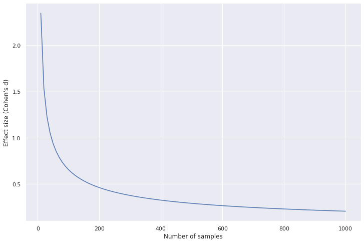
Effect size needed decreases as sample size increases
Code to generate the plot
import statsmodels.api as sm
import numpy as np
import matplotlib.pyplot as plt

tpower = sm.stats.TTestIndPower()
samples = np.linspace(10, 1000, 100)
effect_sizes = [tpower.solve_power(effect_size=None, nobs1=s/2,
                                   alpha=0.05, power=0.9)
                for s in samples]

plt.plot(samples, effect_sizes)

plt.xlabel('Number of samples')
plt.ylabel("Effect size (Cohen's d)")
As sample size increases, the effect size the test can discriminate against decreases, yielding a statisticly significant result. However, it is important to remember:
- A statisticly significant result may not be scientifically or practically significant. The size of the effect is important when considering significance
- The significance threshold and p-value are about the probability of observing this sample of data given the null hypothesis which is different from the probability of the null hypothesis given the data.
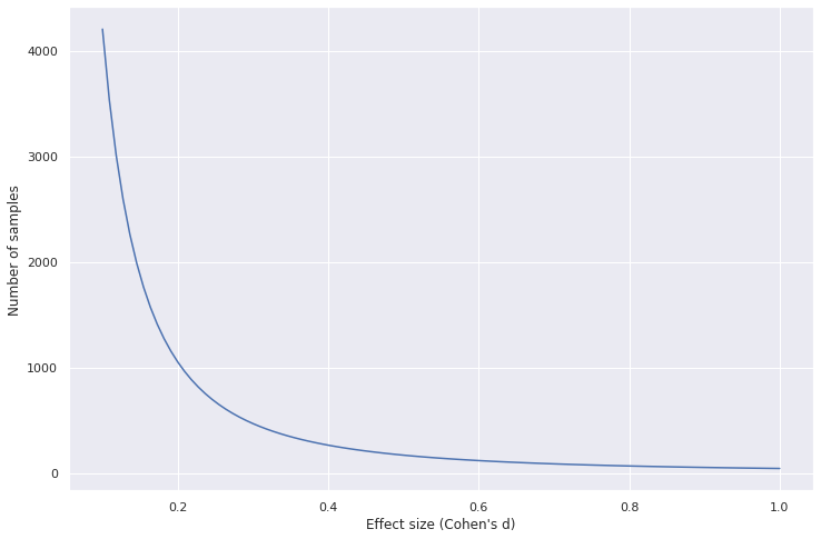
Sample size needed decreases as effect size increases
Code to generate the plot
import statsmodels.api as sm
import numpy as np
import matplotlib.pyplot as plt

tpower = sm.stats.TTestIndPower()
effect_sizes = np.linspace(0.1, 1, 100)
samples_needed = [2*tpower.solve_power(effect_size=es, nobs1=None,
                                       alpha=0.05, power=0.9)
                  for es in effect_sizes]

plt.plot(effect_sizes, samples_needed)

plt.xlabel("Effect size (Cohen's d)")
plt.ylabel('Number of samples')
As the effect size increases the number of samples needed for a statistically significant result decreases drastically. As an example, it is very obvious to tell that NBA basketball players have a different height distribution than the average American. It is much harder to tell whether people from NYC have a different mean height than people from Boston.
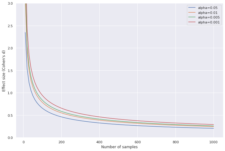
Effect size and sample size needed increases as significance threshold decreases
Code to generate the plot
import statsmodels.api as sm
import numpy as np
import matplotlib.pyplot as plt

tpower = sm.stats.TTestIndPower()

samples = np.linspace(10, 1000, 100)
alphas = [0.05, 0.01, 0.005, 0.001]
alpha_to_effect_sizes = [[tpower.solve_power(effect_size=None, nobs1=s/2,
                                             alpha=a, power=0.9)
                         for s in samples]
                         for a in alphas]

for i, a in enumerate(alphas):
    plt.plot(samples, alpha_to_effect_sizes[i], label='alpha={}'.format(a))
plt.xlabel('Number of samples')
plt.ylabel("Effect size (Cohen's d)")
plt.legend()
plt.ylim((0,3))
As we decrease the significance threshold, we need either a larger effect or more samples to meet the new threshold. This can be understood as, more evidence is required to be more certain.
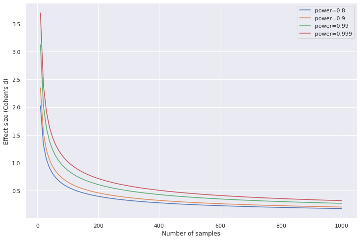
Effect size and sample size needed increases as desired power increases
Code to generate the plot
import statsmodels.api as sm
import numpy as np
import matplotlib.pyplot as plt

tpower = sm.stats.TTestIndPower()

samples = np.linspace(10, 1000, 100)
powers = [0.8, 0.9, 0.99, 0.999]
power_to_effect_sizes = [[tpower.solve_power(effect_size=None, nobs1=s/2,
                                             alpha=0.05, power=p)
                         for s in samples]
                         for p in powers]

for i, p in enumerate(powers):
    plt.plot(samples, power_to_effect_sizes[i], label='power={}'.format(p))
plt.xlabel('Number of samples')
plt.ylabel("Effect size (Cohen's d)")
plt.legend()
As we increase the desired power, we need either a larger effect or more samples to meet the new threshold. Similar to having a stricter significance threshold, more evidence is needed to be more certain.